Efficient Modeling of Tight-Binding Models on Hyperbolic Lattices

Table of Contents

• Overview
• Installation
• Getting Started

Overview

The task of modeling tight-binding models on hyperbolic lattices is split into two steps:

1. Constructing the lattice/model graph For finite systems, this includes the construction of appropriate periodic boundary conditions, while for infinite systems, the corresponding primitive cell and successive supercells are constructed in order to apply the supercell method for hyperbolic band theory. This part is implemented in the GAP package HyperCells. Additionally, the package determines maximally-symmetric Wyckoff positions and simplifies dealing with translation and point group symmetries on the hyperbolic lattice. The package also allows the definition of the graph underlying a specific model, i.e., selecting specific Wyckoff positions, nearest or next-nearest neighbors etc.
2. Defining tight-binding models and using hyperbolic band theory The second package, a Mathematica package called HyperBloch provides functions for importing and easily visualizing the clusters, supercells, and model graphs. Additionally, it allows the user to easily define tight-binding models ontop of the model graph, by placing orbitals at vertices and definining hopping matrices on the edges. Finally, the Abelian Bloch Hamiltonian for the defined model is constructed and thus allows to study eigenstates and eigenvalues.

Note that the output of the HyperCells package, i.e., the cell and model graphs can be read by any programming language, such that using the HyperBloch package is not strictly necessary. The file format definitions can be found in the documentation.

Supercell Method

Hyperbolic lattices were recently theoretically described by a non-Abelian generalization of the Bloch theorem, but practical approaches for efficient computations have remained missing. Our proposed “supercell method” overcomes the challenges posed by noncommuting translations, and enables significant progress towards an analytical description of hyperbolic lattice models in momentum space. Specifically, we use computational group theory to create a sequence of progressively larger unit cells, each formed as a symmetric aggregate of smaller unit cells. We apply the previously established Abelian hyperbolic band theory — which ignores the noncommutativity of translations — to those growing supercells and obtain a converging description of the infinite lattice.

An introduction to the relevant concepts, can be found in Chapter 9 and 10 of the doctoral thesis

P. M. Lenggenhager, Emerging avenues in band theory: multigap topology and hyperbolic lattices, PhD thesis, ETH Zurich, 10.3929/ethz-b-000645370 (2023)

or in the article

P. M. Lenggenhager, J. Maciejko, and T. Bzdušek, Non-Abelian hyperbolic band theory from supercells, Phys. Rev. Lett. 131, 226401 (2023)

Installation

HyperCells

Prerequisite: GAP version 4.11+

First install GAP by following the instructions on the GAP website. In most cases, this boils down to the following steps (to be executed in the directory where GAP should be installed to):

sudo apt-get install build-essential autoconf libtool libgmp-dev libreadline-dev zlib1g-dev
wget https://github.com/gap-system/gap/releases/download/v4.12.2/gap-4.12.2.tar.gz
tar -zxf gap-4.12.2.tar.gz
cd gap-4.12.2/
./configure
make
cd pkg
../bin/BuildPackages.sh
cd ..

You might want to link the executable to ~/bin/gap:

ln -s gap-4.12.2/gap ~/bin/gap

and add ~/bin/ to your path if you have not done so yet:

echo "export PATH=\"$PATH:~/bin\"" >> ~/.bashrc

The HyperCells package is most easily installed by simply cloning the git repository in the user’s GAP package directory:

mkdir -p ~/.gap/pkg
cd ~/.gap/pkg
git clone https://github.com/patrick-lenggenhager/HyperCells.git

To update it to the most recent version, simply pull:

cd ~/.gap/pkg/HyperCells
git pull

HyperBloch

Prerequisites/Dependencies:

• Wolfram Language Interpreter such as Wolfram Language Engine or Mathematica with Wolfram Language 12+ (13+ is recommended)
• NCAlgebra package (version 6+)

Assuming a Wolfram Language Interpreter is already installed, we first install its dependency NCAlgebra

PacletInstall["https://github.com/NCAlgebra/NC/blob/master/NCAlgebra-6.0.3.paclet?raw=true"];

and then the package itself as a paclet:

PacletInstall["https://github.com/patrick-lenggenhager/HyperBloch/releases/download/v0.9.0/PatrickMLenggenhager__HyperBloch-0.9.0.paclet"]

If necessary, update the version number to match the one of the latest release. Alternatively, download the release file manually, and install it with PacletInstall["path"] by passing the path to the downloaded file as argument.

Getting Started

HyperCells

To use the package, start gap and then load the package with

gap> LoadPackage("HyperCells");

A basic example including explanations can be found in the documentation, while more complicated examples, reproducing all our results from the paper can be found in the Supplementary Data and Code.

HyperBloch

To use the package, load it using the command

<< PatrickMLenggenhager`HyperBloch`

A tutorial can be found in the documentation center, which can be opened with the command:

Documentation`HelpLookup["PatrickMLenggenhager/HyperBloch/tutorial/BasicUsage"];

More examples can be found in the specific function pages, for an overview, see

Documentation`HelpLookup["PatrickMLenggenhager/HyperBloch/guide/HyperBlochPackage"];

Again, the more complicated examples, reproducing all our results from the paper, can be found in the Supplementary Data and Code.

Worked-Out Example

The below example is taken from the Supplementary Data and Code and demonstrates the necessary steps to find the density of states of an elementary nearest-neighbor hopping model on the \(\{8,8\}\) lattice.

In GAP, we first construct the primitive cell, then the model graph (based on the tessellation graph), and finally the 2-supercell:

# load the HyperCells package
LoadPackage( "HyperCells" );

# set up (proper) triangle group
tg := ProperTriangleGroup( [ 2, 8, 8 ] );

# specify the quotient defining the primitive cell
qpc := TGQuotient( [ 2, 6 ] );

# construct symmetric primitive cell
cgpc := TGCellGraph( tg, qpc, 3 : simplify := 5 );
Export( cgpc, "(2,8,8)_T2.6_3.hcc" ); # export

# elementary nearest-neighbor model
model := TessellationModelGraph( cgpc, true : simplify := 5 );
Export( model, "{8,8}-tess_T2.6_3.hcm" ); # export

# construct symmetric supercell
sc := TGCellSymmetric( tg, TGQuotient( [ 3, 11 ] ), 3 );

# extend the model defined on the primitive cell to the supercell
scmodel := TGSuperCellModelGraph( model, sc : simplify := 0 );
Export( scmodel, "{8,8}-tess_T2.6_3_sc-T3.11.hcs" ); # export

Next, in Mathematica, we load the package

<< PatrickMLenggenhager`HyperBloch`

and then the exported data:

SetDirectory[NotebookDirectory[]];

pcell = ImportCellGraphString[Import["(2,8,8)_T2.6_3.hcc"]];
pcmodel = ImportModelGraphString[Import["{8,8}-tess_T2.6_3.hcm"]];
scmodel = ImportSupercellModelGraphString[Import["{8,8}-tess_T2.6_3_sc-T3.11.hcs"]];

Note the use of the Import[] function inside the ImportCellGraphString[] function. This is necessary, because the exported file is a text file, which contains the string representation of the cell graph. The Import[] function is used to read the file, while the ImportCellGraphString[] function is used to parse the string and construct the cell graph. The same applies to the ImportModelGraphString[] and ImportSupercellModelGraphString[] functions. Alternatively, we could have used the function ExportString() in GAP to export the cell graph as a string, copied the string into a Mathematica notebook, and then used the ImportCellGraphString[] function (or one of the analogous functions) directly to parse the string and construct the cell graph.

The HyperBloch package provides convenient functions for visualizing the model:

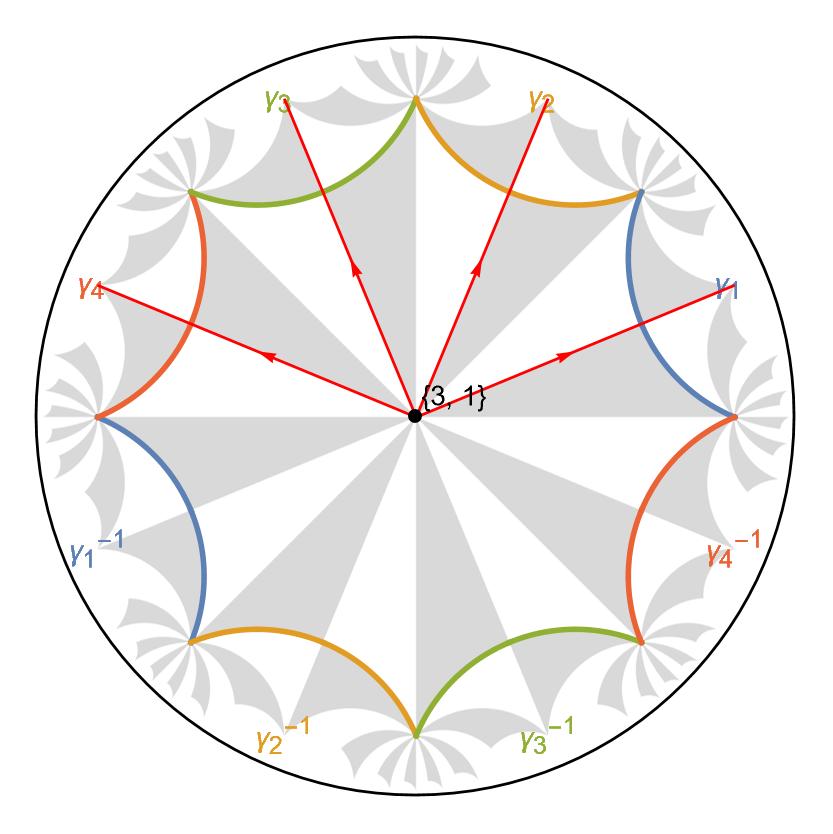
VisualizeModelGraph[pcmodel,
	Elements -> <|
		ShowCellGraphFlattened -> {},
		ShowCellBoundary -> {ShowEdgeIdentification -> True}
	|>,
	CellGraph -> pcell,
	NumberOfGenerations -> 2,
	ImageSize -> 300
]

producing the following output:

To construct the Abelian Bloch Hamiltonian for the given model, we use

FullSimplify[AbelianBlochHamiltonianExpression[pcmodel, 1, 0 &, -1 &, k]]

which results in

{ { -2 (Cos[k[1]] + Cos[k[2]] + Cos[k[3]] + Cos[k[4]]) } }

For more efficient evaluation, we precompile the Bloch Hamiltonian by specifying the option CompileFunction->True:

Hpc = AbelianBlochHamiltonian[pcmodel, 1, 0 &, -1 &, CompileFunction -> True];

To compute the density of states (DOS), we can now take advantage of the independence of different momentum sectors and therefore parallelize it:

ComputeDOS[cfH_, Npts_, Nruns_, {Emin_, Emax_}, dE_] := 
 Module[{data, tot, dimk = Length[cfH[[2]]]},
  data = 
   Transpose[{MovingAverage[Range[Emin, Emax, dE], 2], 
     Total@ParallelTable[
       HistogramList[
         Flatten@Table[
           Chop@Eigenvalues[cfH @@ RandomReal[{-Pi, Pi}, dimk]], {i, 
            1, Round[Npts/Nruns]}], {Emin, Emax, dE}][[2]], {j, 1, 
        Nruns}, Method -> "FinestGrained"]}];
  tot = Total@data[[;; , 2]];
  {#1, #2/dE/tot} & @@@ data
  ]
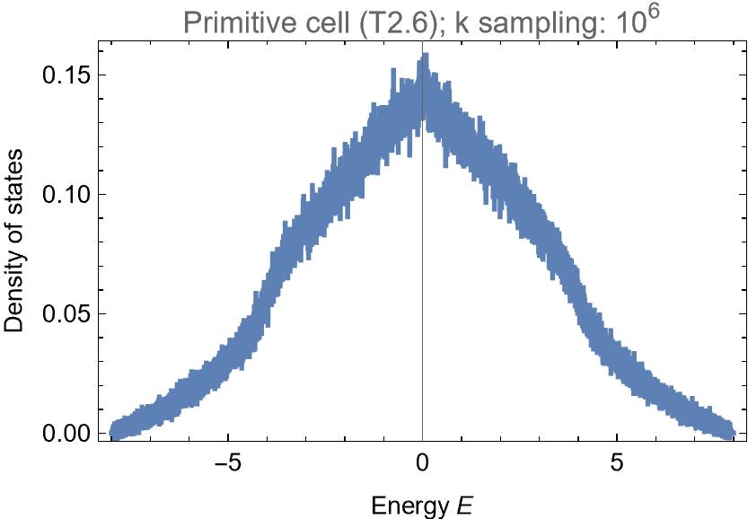
dospc = ComputeDOS[Hpc, 10^6, 32, {-8 - 0.005, 8}, 0.005];

We find:

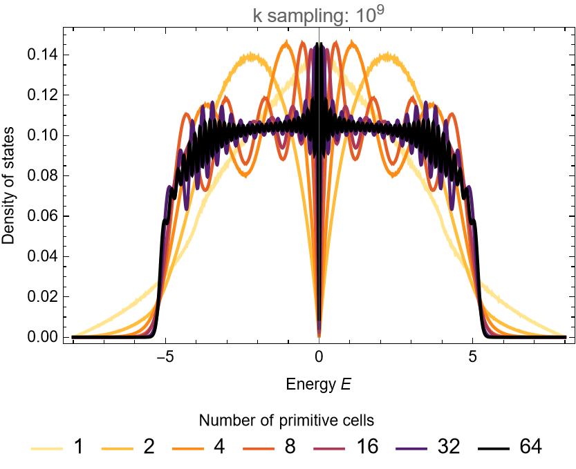
It is just as easy to apply the supercell method. For example, constructing the Abelian Bloch Hamiltonian on the larger supercell, which thus captures some of the higher-dimensional irreducible representations on the original primitive cell, and computing the resulting DOS can be done as follows:

Hsc = AbelianBlochHamiltonian[scmodel, 1, 0 &, -1 &, PCModel -> pcmodel, CompileFunction -> True];
dossc = ComputeDOS[Hsc, 10^4, 32, {-8 - 0.005, 8}, 0.005];

Performing the computations with higher momentum-resolution (\(10^9\) points) and for more supercells (up to 64 primitive cells), we can nicely observe the convergence of the DOS: